Doppler models

Latest Doppler Fit Model for ARGOS-2 Data

If you're looking for the super hyper advanced data fit routine for Project Desert Tortoise then you want the matlab file below! Otherwise, read on to learn more about Doppler and his amazing discovery of velocity based frequency shifting!

http://wiki.nebarnix.com/wiki/File:Doppler3DRotationInclination3FitandWebephem.m

Understanding Doppler Shifts

Who is Doppler?

Taken from Wikipedia,

Christian Andreas Doppler (/ˈdɒplər/; German: [ˈdɔplɐ]; 29 November 1803 – 17 March 1853) was an Austrian mathematician and physicist. He is celebrated for his principle — known as the Doppler effect — that the observed frequency of a wave depends on the relative speed of the source and the observer. He used this concept to explain the color of binary stars.

What is a Doppler Shift?

We should all be familiar with the sound of a passing car, airplane, or even more dramatic, passing ambulance. The sound changes as the object rushes by us. The pitch becomes lower, sometimes dramatically depending on how close we are and how fast (and in which direction) the object is moving. We can model this using math!

It turns out, the same thing happens to electromagnetic waves that happens to sound waves -- including radio and even light waves, as our friend Dr. Doppler discovered, where binary stars appear to change color slightly as they orbit around each other.

Doppler shifting is caused by the compression of the waves emitted from a source. For audio waves it is the physical objecting 'catching up' with waves emitted. Sound waves always travel at a constant velocity (speed of sound), so you can 'catch up' with the waves moving in front of, and 'leave behind' the waves emitted backwards. As the space betweeen the waves changes, their frequency changes because frequency is defined by the number of changes of the wave per unit time. More changes per unit distance means you hear the vibrations faster, less changes per unit time means you hear the vibrations slower. Wikipedia has several articles to make this more understandable. For electromagnetic waves, it is actually time compression of the source, but it can be modeled as the same effect with the same equations.

Project Desert Tortoise will uses these models to perform geolocation of radio transmitters based their change in frequency as heard by the passing spacecraft. This also could be used to determine your location based on the changing frequency of a passing spacecraft, which is exactly how it was done before GPS came along. GPS is a much better solution, but has its own set of challenges (it won't work on Mars, for example).

Linear Case

Let's start simple. We have a road and there is an observer (A) standing at some distance d from this road. A car (B) is traveling at a constant velocity v. Let us assume that it is emitting engine noise at frequency ftx. The road is straight, and so we will use Cartesian (x and y) coordinates for this example.

The distance between them is just the Pythagorean Theorem, which is the distance formula.

Or in the full expanded form



Now what is the relative velocity between these two points? It is simply the rate of change of the distance. If you don't know calculus, this is a GREAT example of just how powerful it can be. Luckily, we can take what is called a derivative -- which is exactly the rate of change of a formula and we can use Wolfram Alpha to do the hard work for us. Seriously. Click the link or type "derivative of sqrt{(A1-(v*t+B1))^2+(A2-B2)^2} with respect to t" into the box on the main page. It will spit the following back at you.




Now that we have the formula for relative velocity of an object moving at a constant speed along the x axis, let's plot an example with the following parameters (you are standing 5 meters from the road and the car moving from -10 to +10 meters along the road at 1 meter per second).

and

Relative Distance Between the car and the observer as a function of time:
http://www.wolframalpha.com/input/?i=plot+sqrt%7B%280-%281*t%2B-10%29%29%5E2%2B%280-5%29%5E2%7D+from+0+to+20

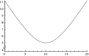
Relative Velocity Between the car and the observer as a function of time:
http://www.wolframalpha.com/input/?i=plot+%28%280-%28-10%29-x%29%29%2Fsqrt%28%280-%28-10%29-x%29%5E2%2B%280-5%29%5E2%29+x+from+0+to+20



We're almost there. The formula for the doppler shift of an emitted frequency is on the wikipedia article where ft is the transmitted frequency and c is the speed of waves in the medium (in this case, the speed of sound in air)




So this makes our final (huff puff!) equation!



Assume engine noise Ftx = 3khz and c = 343 m/sec (at standard conditions)
Plotting this (Wolfram Alpha "plot (2*3000*((0-(-10)-x))/sqrt((0-(-10)-x)^2+(0-5)^2))/343 x from 0 to 20") shows the final received frequency over time! YAY! NEEEEEEEEOoowwwww!!! Except our car is traveling a whopping 1 meter per second, so the doppler is only 15Hz. Feel free to imagine that this is 150Hz and the car is moving at 10m/sec.

http://www.wolframalpha.com/input/?i=plot+%282*3000*%28%280-%28-10%29-x%29%29%2Fsqrt%28%280-%28-10%29-x%29%5E2%2B%280-5%29%5E2%29%29%2F343+x+from+0+to+20



This relationship is linear as long as the car stays below some fraction of the speed of sound (Hopefully!). If we wish to assume that the car can go REALLY fast, we need to use the expanded form of the doppler equation which is left up to the reader and Wolfram Alpha:

Animation

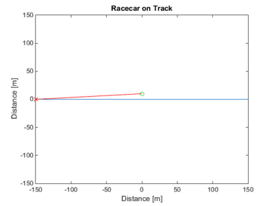
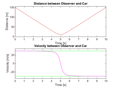
I came up with an animation to demonstrate the result an maybe an easier to digest way. I went ahead and speeded up the racecar to a more appropriate speed:

RoadLength = 300;   %A 300 meter section of road
RaceCarSpeed = 30; %30 m/s is a little more than 100km/hr VRRRRRRROOOMMM! (constant velocity)
ObsRoadDistance = 10; %Let's stand 10m from the side of the road

Full Matlab Code for Racecar Math: (click expand)->

%% 2D linear Relative Velocity (constant velocity)
%using meters, seconds, and radians (2*pi radians = 360 degrees = 1 circle)
clear all;

RoadLength = 300;   %A 300m section of road
RaceCarSpeed = 30; %30 m/s is a littl more than 100km/hr VRRRRRRROOOMMM! (constant velocity)
RaceCarTime = RoadLength/RaceCarSpeed; %how long it will take to drive 1000m at 30m/s

ObsRoadDistance = 10; %Let's stand 10m from the side of the road

t=0:RaceCarTime/100:RaceCarTime; %Drive along the road until the end

%Plot the road, the starting point of the car, and the observer
figure(1);
plot([-RoadLength/2 RoadLength/2],[0 0],-RoadLength/2,0,'Xr',0,ObsRoadDistance,'Og');
Dt = sqrt((0-(RaceCarSpeed*t-RoadLength/2)).^2+(ObsRoadDistance-0)^2);
Vt = (RaceCarSpeed*(0-(-RoadLength/2)-t.*RaceCarSpeed))./Dt;
axis([-RoadLength/2 RoadLength/2 -RoadLength/2 RoadLength/2]);
title('Racecar on Track');


%Plot the distance between the car and the observer
figure(2);
subplot(3,1,1);
plot(t,Dt);
axis('tight');
set(gca,'Ylim',[0 max(Dt)+10]);
title('Distance between Observer and Car');


%Plot the velocity between the car and the observer, and also put bars on
%the racecar max and min possible velocities
subplot(3,1,2);
plot(t,-RaceCarSpeed*ones(numel(t),1),'g',t,RaceCarSpeed*ones(numel(t),1),'g',t,Vt);
title('Velocity between Observer and Car');
axis('tight');
set(gca,'Ylim',[-(RaceCarSpeed+5) (RaceCarSpeed+5)]);

%Doppler
c = 299792; %in km per second
Ft = 401.65e6; %401.65Mhz uplink freq
F =(2*Vt*Ft)./(c-Vt);
subplot(3,1,3);
plot(t,F);
title('Doppler Shift of Observer (at 401Mhz)');
axis('tight');

And the Animation

%% Animate
%plot the center point, the circle of the track, the starting point of the
%car, and the observer
filename = 'RaceCarRoad.gif';
filename2 = 'RaceCarRoad2.gif';

Dt = sqrt((0-(RaceCarSpeed*t-RoadLength/2)).^2+(ObsRoadDistance-0)^2);
Vt = (RaceCarSpeed*(0-(-RoadLength/2)-t.*RaceCarSpeed))./Dt;
    
for T=0:.1:max(t)
    %Plot the distance between the car and the observer
    figure(2);
    subplot(2,1,1);
    plot(t,Dt,'r',[T T],[0 Dt(find(T<t,1))],'r');
    axis('tight');
    set(gca,'Ylim',[0 max(Dt)+5]);
    title('Distance between Observer and Car');
    xlabel('Time [s]');
    ylabel('Distance [m]');
    
    %Plot the velocity between the car and the observer, and also put bars on
    %the racecar max and min possible velocities
    subplot(2,1,2);
    plot([0 max(t)],[-RaceCarSpeed -RaceCarSpeed],'g',[0 max(t)],[RaceCarSpeed RaceCarSpeed],'g',t,Vt,'m',[T T],[-100 100],'-.r');
    title('Velocity between Observer and Car');
    axis('tight');
    set(gca,'Ylim',[-(RaceCarSpeed+5) (RaceCarSpeed+5)]);
    xlabel('Time [s]');
    ylabel('Velocity [m/s]');
    
    %Output frame to gif
    drawnow
    frame = getframe(get(gcf,'Number'));
    
    im = frame2im(frame);
    [imind,cm] = rgb2ind(im,16);    
    
    if T == 0
        imwrite(imind,cm,filename2,'gif', 'Loopcount',inf);
    else
        imwrite(imind,cm,filename2,'gif','WriteMode','append','DelayTime',0.1);
    end
    
    figure(1);
    plot([-RoadLength/2 RoadLength/2],[0 0],RaceCarSpeed*T-(RoadLength/2),0,'Xr',0,ObsRoadDistance,'Og',[RaceCarSpeed*T-(RoadLength/2) 0],[0 ObsRoadDistance],'r');
    
    axis([-RoadLength/2 RoadLength/2 -RoadLength/2 RoadLength/2]);
    title('Racecar on Track');
    xlabel('Distance [m]');
    ylabel('Distance [m]');
    
    %Output frame to gif
    drawnow
    frame = getframe(get(gcf,'Number'));
    
    im = frame2im(frame);
    [imind,cm] = rgb2ind(im,16);    
    
    if T == 0
       imwrite(imind,cm,filename,'gif', 'Loopcount',inf);
    else
       imwrite(imind,cm,filename,'gif','WriteMode','append','DelayTime',0.1);
    end
end

Circular Case

It is clear that this picture does not work for a satellite. A satellite is not traveling along a linear path, instead, a circle. Let's follow the same idea but close the track from a country road into a racetrack where the cars are traveling in a circle.

We can use the same variables, but now we can reference everyone against the center of the track instead of using the observer as the origin. The same car B is traveling at the same constant velocity v on a track with a radius Rb while our observer A is at distance Ra from the center of the track, and an angle Atheta. We are doing away with the above notation because it takes forever and Matlab is so nice! We can still use Wolfram Alpha for calculus and plotting. Note that from here on out we will switch from audio to radio waves (from speed of sound in air to speed of light) and we will be using the expanded doppler formula because satellites move REALLY fast.

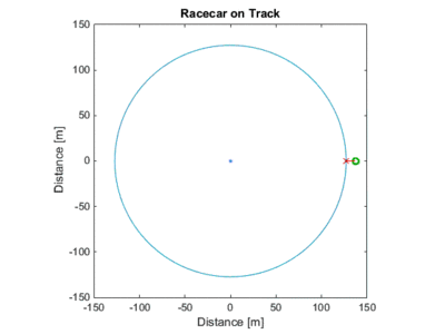
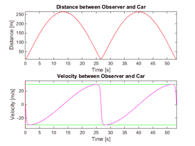
The case for the viewer outside the track. Notice how the relative velocity will always reach the speed of the car, because the car is, for an instant, 'pointed' directly at the observer (A tangent intersects the observer)

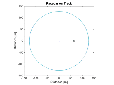
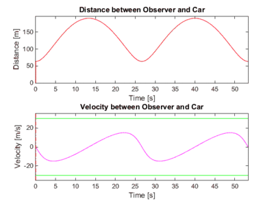
The case for the viewer inside the track. Note that the relative velocity is always less than the speed of the car, because the car is never 'pointed' at the observer.

Full Matlab Code for the Circular Case (click expand)->

%% 2D circular Relative Velocity
%using meters, seconds, and radians (2*pi radians = 360 degrees = 1 circle)
clear all;

TrackLength = 800;   %A really short track of 800 meters
RaceCarSpeed = 30; %30 m/s is a littl more than 100km/hr VRRRRRRROOOMMM!
RaceCarLapTime = TrackLength/RaceCarSpeed; %Distance / Velocity = Time

TrackRadius = TrackLength /(2*pi); % circumference = 2*pi*radius
RaceCarAngularVelocity = (2*pi)/RaceCarLapTime; %Angular velocity is degrees/second (or radians/second)

%Case 1, standing at the center
ObsTrackDistance = -TrackRadius; %Let's stand in the center of the track
%Case 2, standing in the grandstands
ObsTrackDistance = 10; %Let's stand 10 meters outside the track
%Case 3, standing in the pit
%ObsTrackDistance = -10; %Let's stand 10 meters inside the track

ObsRadius = TrackRadius+ObsTrackDistance;

t=0:RaceCarLapTime/100:2*RaceCarLapTime; %2 laps around the track, evaluate solution 100 times per lap
InitialAngle = 0; %Starting point of the car on the track

%plot the center point, the circle of the track, the starting point of the
%car, and the observer
figure(1);
plot(0,0,'.b',TrackRadius*cos(0:0.01:2*pi),TrackRadius*sin(0:0.01:2*pi),TrackRadius*cos(InitialAngle),TrackRadius*sin(InitialAngle),'Xr',ObsRadius,0,'Og');
Dt = sqrt(ObsRadius^2+TrackRadius^2-2*ObsRadius*TrackRadius.*cos(InitialAngle+RaceCarAngularVelocity.*t));
Vt = -(ObsRadius*TrackRadius*RaceCarAngularVelocity.*sin(InitialAngle+RaceCarAngularVelocity.*t))./(sqrt(ObsRadius^2+TrackRadius^2-2*ObsRadius*TrackRadius.*cos(InitialAngle+RaceCarAngularVelocity.*t)));
pbaspect([1 1 1])
title('Racecar on Track');


%Plot the distance between the car and the observer
figure(2);
subplot(3,1,1);
plot(t,Dt);
axis('tight');
title('Distance between Observer and Car');


%Plot the velocity between the car and the observer, and also put bars on
%the racecar max and min possible velocities
subplot(3,1,2);
plot(t,-RaceCarSpeed*ones(numel(t),1),'g',t,RaceCarSpeed*ones(numel(t),1),'g',t,Vt);
title('Velocity between Observer and Car');
axis('tight');
set(gca,'Ylim',[-(RaceCarSpeed+5) (RaceCarSpeed+5)]);

%Doppler
c = 299792; %in km per second
Ft = 401.65e6; %401.65Mhz uplink freq
F =(2*Vt*Ft)./(c-Vt);
subplot(3,1,3);
%plot(t,F,xdata,Fscale*ydata+Foffset,'-o');
plot(t,F);
title('Doppler Shift of Observer (at 401Mhz)');
axis('tight');

Animation Code

%% Animate
%plot the center point, the circle of the track, the starting point of the
%car, and the observer
filename = 'RaceCarPit.gif';
filename2 = 'RaceCarPit2.gif';

for T=0:.25:max(t)
    %Plot the distance between the car and the observer
    figure(2);
    subplot(2,1,1);
    plot(t,Dt,'r',[T T],[0 Dt(find(T<t,1))],'r');
    axis('tight');
    set(gca,'Ylim',[0 max(Dt)+5]);
    title('Distance between Observer and Car');
    xlabel('Time [s]');
    ylabel('Distance [m]');
    
    %Plot the velocity between the car and the observer, and also put bars on
    %the racecar max and min possible velocities
    subplot(2,1,2);
    plot([0 max(t)],[-RaceCarSpeed -RaceCarSpeed],'g',[0 max(t)],[RaceCarSpeed RaceCarSpeed],'g',t,Vt,'m',[T T],[-100 100],'-.r');
    title('Velocity between Observer and Car');
    axis('tight');
    set(gca,'Ylim',[-(RaceCarSpeed+5) (RaceCarSpeed+5)]);
    xlabel('Time [s]');
    ylabel('Velocity [m/s]');
    
    %Output frame to gif
    drawnow
    frame = getframe(get(gcf,'Number'));
    %frame.cdata = frame.cdata(1:2:end,1:2:end,:);
    im = frame2im(frame);
    [imind,cm] = rgb2ind(im,16);    
    
    if T == 0
        imwrite(imind,cm,filename2,'gif', 'Loopcount',inf);
    else
        imwrite(imind,cm,filename2,'gif','WriteMode','append','DelayTime',0.1);
    end
    
    figure(1);
    plot(0,0,'.b',TrackRadius*cos(0:0.01:2*pi),TrackRadius*sin(0:0.01:2*pi),TrackRadius*cos(InitialAngle+RaceCarAngularVelocity.*T),TrackRadius*sin(InitialAngle+RaceCarAngularVelocity.*T),'Xr',ObsRadius,0,'Og',[TrackRadius*cos(InitialAngle+RaceCarAngularVelocity.*T) ObsRadius],[TrackRadius*sin(InitialAngle+RaceCarAngularVelocity.*T) 0],'r');
    Dt = sqrt(ObsRadius^2+TrackRadius^2-2*ObsRadius*TrackRadius.*cos(InitialAngle+RaceCarAngularVelocity.*t));
    Vt = -(ObsRadius*TrackRadius*RaceCarAngularVelocity.*sin(InitialAngle+RaceCarAngularVelocity.*t))./(sqrt(ObsRadius^2+TrackRadius^2-2*ObsRadius*TrackRadius.*cos(InitialAngle+RaceCarAngularVelocity.*t)));
    pbaspect([1 1 1])
    title('Racecar on Track');
    xlabel('Distance [m]');
    ylabel('Distance [m]');
    
    %Output frame to gif
    drawnow
    frame = getframe(get(gcf,'Number'));
    %frame.cdata = frame.cdata(1:2:end,1:2:end,:);
    im = frame2im(frame);
    [imind,cm] = rgb2ind(im,16);    
    
    if T == 0
        imwrite(imind,cm,filename,'gif', 'Loopcount',inf);
    else
        imwrite(imind,cm,filename,'gif','WriteMode','append','DelayTime',0.1);
    end
end

Polar Spherical Case

The circular case models what happens when a satellite passes DIRECTLY over you, but cannot account for what happens when there is an offset to one side of the pass. We can only model this case by moving forward to spherical coordinates. Things get a little messy here, but we will use the exact same approaches we used before -- the equations are just a little longer because we have to account for the new third axis, represented by the unit vector Phi. We will use the standard where phi represents rotation along the equator and theta represents the angle between the north pole and the vector while r is again the radius.

This case models how a satellite travels quite well, and in fact is almost enough to solve our problem. We could model a 90 degree inclination orbit, which is representative of any other circular orbit passing directly overhead. We can probably even use this model to solve for geo-locations within about 250km which isn't bad for a 'rough guess'.

What is that 250km all about? Well unfortunately this is the distance that a point will move along the equator during a 15 minute satellite pass (assuming a sat altitude of 850km). The effect will get better at the pole and worse at the equator, but we really can't ignore this basic fact: the earth turns under the satellites!

Full Matlab Code for the Polar Spherical Case

%% 3D Relative Velocity
%using kilometers and seconds
clear all;
ObsRad        = 6378; %sea level
%ObsTheta      = 1.74;
ObsTheta      = pi/2; %equator
%ObsPhi        = 0.135;
ObsPhi        = 0 ; %0 is directly under, pi/2 is as far as you can get

SatRad        = ObsRad + 854; %sea level + altitude
SatPhi        = 0;       %Phi of sat is zero, vary pass height by observer phi
SatTheta      = pi/2;    %Initial position of 0 (equator)
OrbitalPeriod = 6127.2;  %102 minutes to seconds
OrbitalLength = 2*pi*SatRad;
SatSpeed = OrbitalLength/OrbitalPeriod;
SatAngularVel = 2*pi/OrbitalPeriod; 

t=0:OrbitalPeriod/1000:2*OrbitalPeriod; %2 orbits

Vt_num = (ObsRad*SatRad*SatAngularVel*(sin(ObsTheta)*cos(SatPhi-ObsPhi)*cos(SatAngularVel*t+SatTheta)-cos(ObsTheta)*sin(SatAngularVel*t+SatTheta)));
%Vt_num = -(ObsRad*SatRad*(SatAngularVel*sin(SatTheta + SatAngularVel*t)*cos(ObsTheta) - SatAngularVel*cos(SatTheta + SatAngularVel*t)*sin(ObsTheta)*cos(ObsPhi - SatPhi)));
Vt_den = sqrt(ObsRad^2+SatRad^2-2*ObsRad*SatRad*(sin(SatTheta+SatAngularVel*t)*sin(ObsTheta)*cos(SatPhi-ObsPhi)+cos(SatTheta+SatAngularVel*t)*cos(ObsTheta)));
%Vt_den = sqrt(ObsRad^2 + SatRad^2 - 2*ObsRad*SatRad*(cos(SatTheta + SatAngularVel*t)*cos(ObsTheta) + sin(SatTheta + SatAngularVel*t)*sin(ObsTheta)*cos(ObsPhi - SatPhi)));
Vt = Vt_num ./ Vt_den;

subplot(3,1,1);
plot(t,Vt_den);
title('Distance to Observer');

subplot(3,1,2);
plot([0 max(t)],[SatSpeed SatSpeed],'g',[0 max(t)],[-SatSpeed -SatSpeed],'g',t,Vt);
axis([0 max(t) -SatSpeed*1.2 SatSpeed*1.2]);
title('Velocity to Observer');

%%Doppler
c = 299792; %in km per second
Ft = 401.65e6; %401.65Mhz uplink freq
F =(2*Vt*Ft)./(c-Vt);
subplot(3,1,3);
plot(t,F);
title('Doppler Shift of Observer (at 401Mhz)');

Animation Code Placeholder

Polar Spherical Case with Rotating Earth

This is a simple modification. We can just make phi of the observer also time dependent then re-calculate the derivative. The curve changes shape noticeably, which is expected because 250 km is no small distance.

Full Matlab Code for the Polar Spherical Case

%% 3D Relative Velocity with Earth's Rotation
%derivative of sqrt(A1^2+B1^2-2*A1*B1*(sin (v*t+A2)*sin (B2)*cos (A3-(v2*t+B3))+cos (v*t+A2)*cos (B2))) with respect to t
%(d)/(dt)(sqrt(A1^2+B1^2-2 A1 B1 (sin(v t+A2) sin(B2) cos(A3-(v2 t+B3))+cos(v t+A2) cos(B2)))) = -(A1 B1 (v2 sin(B2) sin(A2+t v) sin(A3-B3-t v2)+v sin(B2) cos(A2+t v) cos(A3-B3-t v2)-v cos(B2) sin(A2+t v)))/sqrt(A1^2-2 A1 B1 (sin(B2) sin(A2+t v) cos(A3-B3-t v2)+cos(B2) cos(A2+t v))+B1^2)
%A1 is sat radius => SatRad
%v is sat angular velocity = SatAngularVel
%A2 is sat theta start = SatTheta
%A3 is sat phi => SatPhi

%B1 is obs radius => ObsRad
%B2 is obs theta => ObsTheta
%B3 is obs phi start => ObsPhi
%v2 is obs angular velocity => ObsAngularVel

ydata = [1506, 1022, 493, -61, -618, -1154, -1648, -2089, -2472, -2798, -3070, -3296, -3482];
xdata = [42.311,72.211,102.4552,132.2255,162.215,192.2178,222.314,252.2178,282.2255,312.2255,342.2255,372.2255,402.2255];

ObsRad = 6368; %center of European pass (50 degrees)
ObsTheta = 1.74;
ObsPhi = 0.135;
SidrealPeriod = 86164; %23 hours 56 minutes and 4 seconds => seconds
ObsAngularVel = 2*pi/SidrealPeriod;  

SatRad = ObsRad + 854; %sea level + altitude
SatPhi = 0; %inclination of 90 (really its 98, but we don't realy have a term for this
SatTheta = pi/2; %Initial position of 0 (equator)
OrbitalPeriod = 6127.2; %102.12 minutes => seconds
SatAngularVel = 2*pi/OrbitalPeriod; 

Fscale = 4.9;
Foffset = 2048;

t = -0.07*OrbitalPeriod : OrbitalPeriod/1000 : 0.07*OrbitalPeriod; %1000 seconds
Vt_num = (SatRad * ObsRad * (ObsAngularVel*sin(ObsTheta).*sin(SatAngularVel*t+SatTheta).*sin(SatPhi-ObsPhi-ObsAngularVel*t)+SatAngularVel*sin(ObsTheta).*cos(SatTheta+SatAngularVel*t).*cos(SatPhi-ObsPhi-t*ObsAngularVel)-SatAngularVel*cos(ObsTheta).*sin(SatTheta+t*SatAngularVel)));
Vt_den = sqrt(ObsRad^2 + SatRad^2 - 2*SatRad*ObsRad*(sin(ObsTheta).*sin(SatAngularVel*t+SatTheta).*cos(SatPhi-ObsPhi-ObsAngularVel*t)+cos(ObsTheta).*cos(SatTheta+SatAngularVel*t)));
Vt = Vt_num ./ Vt_den;

subplot(3,1,1);
plot(t,Vt_den);

TcrossingInterp2= interp1(Vt,t,0);

title(['Distance to Observer: ' num2str(min(Vt_den)) 'km at ' num2str(TcrossingInterp2) 's']);

subplot(3,1,2);
plot(t,Vt);
title('Velocity to Observer');

%%Doppler
c = 299792; %in km per second
Ft = 401.65e6; %401.65Mhz uplink freq
F =(2*Ft*Vt)./(c-Vt);
subplot(3,1,3);
plot(t,F,xdata,Fscale*ydata+Foffset,'-o');
title('Doppler Shift of Observer (at 401Mhz)');
max(F);

Animation Code Place Holder

Variable Inclination Spherical Case with Rotating Earth

Whittling away errors, we have now exposed the next problem. Orbits have inclinations, which means that the earth's angular velocity vector and the satellite's motion vector are no longer orthagonal. During ascending nodes and descending nodes the velocity of the earth slightly adds and subtracts from the relative velocity, and thus each node will have a slightly different shape based on this larger or smaller velocity.

It turns out, this isn't so easy. Our models break down when we try to add some sort of tilt to the axis. I started making circles and ovals and thinking about what an orbit looks like on the XY, YZ, and XZ planes (it looks like a squished circle). I came up with this:

x = (r.*cos(omega.*t+phase));
y = (r.*-cos(inc).*sin(omega.*t+phase));
z = (r.*sin(inc).*sin(omega.*t+phase));

Go ahead, plot this. Its a circular orbit with variable inclination! But now the hard part, we have to transfer this to spherical coordinates to work with the models we want.

If we follow the following transform:

phi = atan2(y,x);
theta = acos(sin(z/(r*sin(theta))));
r = r;

we can arrive at the final answer. we can convert acos to arctan using an identity to make matlab happy (it didn't seem to work with acos)

phi = atan2((-cos(inc)*sin(omega*t+phase)),(cos(omega*t+phase)));
theta = (pi/2.0)-atan2((r*sin(inc)*sin(omega*t+phase)),sqrt((r.*-cos(inc).*sin(omega.*t+phase)).^2 + (r.*cos(omega.*t+phase)).^2));

That makes the distance formula between the observer and the sat:

%Distance formula in spherical coordinates is
%sqrt(r1^2    +r2^2    -2*r1    *r2    *(sin(theta1)*sin(theta2)*cos(phi1-phi2)+cos(theta1)*cos(theta2)))
%D(t) = sqrt(SatRad^2+ObsRad^2-2*SatRad*ObsRad*(sin(((pi/2.0)-atan2((SatRad.*sin(SatInc).*sin(SatAngularVel.*t+SatPhase)),sqrt((SatRad.*-cos(SatInc).*sin(SatAngularVel.*t+SatPhase)).^2 + (SatRad.*cos(SatAngularVel.*t+SatPhase)).^2))))*sin(ObsTheta)*cos(atan2((-cos(SatInc).*sin(SatAngularVel.*t+SatPhase)),(cos(SatAngularVel.*t+SatPhase)))-(ObsAngularVel*t+ObsPhi))+cos(((pi/2.0)-atan2((SatRad.*sin(SatInc).*sin(SatAngularVel.*t+SatPhase)),sqrt((SatRad.*-cos(SatInc).*sin(SatAngularVel.*t+SatPhase)).^2 + (SatRad.*cos(SatAngularVel.*t+SatPhase)).^2))))*cos(ObsTheta)))

If we take the derivative (yes, yes, its VERY ugly due to the use of atan2...) then we arrive at the final formula.

%syms t SatRad ObsRad ObsPhi ObsTheta ObsAngularVel SatInc SatAngularVel ObsAngularVel SatPhase

%diff(sqrt(SatRad^2+ObsRad^2-2*SatRad*ObsRad*(sin(((pi/2.0)-atan2((SatRad.*sin(SatInc).*sin(SatAngularVel.*t+SatPhase)),sqrt((SatRad.*-cos(SatInc).*sin(SatAngularVel.*t+SatPhase)).^2 + (SatRad.*cos(SatAngularVel.*t+SatPhase)).^2))))*sin(ObsTheta)*cos(atan2((-cos(SatInc).*sin(SatAngularVel.*t+SatPhase)),(cos(SatAngularVel.*t+SatPhase)))-(ObsAngularVel*t+ObsPhi))+cos(((pi/2.0)-atan2((SatRad.*sin(SatInc).*sin(SatAngularVel.*t+SatPhase)),sqrt((SatRad.*-cos(SatInc).*sin(SatAngularVel.*t+SatPhase)).^2 + (SatRad.*cos(SatAngularVel.*t+SatPhase)).^2))))*cos(ObsTheta))),t)

%Vt = (ObsRad*SatRad*(sin(ObsPhi - atan2(-sin(SatPhase + SatAngularVel*t)*cos(SatInc), cos(SatPhase + SatAngularVel*t)) + ObsAngularVel*t)*sin(pi/2 - atan2(SatRad*sin(SatPhase + SatAngularVel*t)*sin(SatInc), (SatRad^2*cos(SatPhase + SatAngularVel*t)^2 + SatRad^2*sin(SatPhase + SatAngularVel*t)^2*cos(SatInc)^2)^(1/2)))*sin(ObsTheta)*(ObsAngularVel + ((real(cos(SatPhase + SatAngularVel*t)) + imag(sin(SatPhase + SatAngularVel*t)*cos(SatInc)))^2*((imag(SatAngularVel*sin(SatPhase + SatAngularVel*t)) + real(SatAngularVel*cos(SatPhase + SatAngularVel*t)*cos(SatInc)))/(real(cos(SatPhase + SatAngularVel*t)) + imag(sin(SatPhase + SatAngularVel*t)*cos(SatInc))) - ((real(SatAngularVel*sin(SatPhase + SatAngularVel*t)) - imag(SatAngularVel*cos(SatPhase + SatAngularVel*t)*cos(SatInc)))*(imag(cos(SatPhase + SatAngularVel*t)) - real(sin(SatPhase + SatAngularVel*t)*cos(SatInc))))/(real(cos(SatPhase + SatAngularVel*t)) + imag(sin(SatPhase + SatAngularVel*t)*cos(SatInc)))^2))/((imag(cos(SatPhase + SatAngularVel*t)) - real(sin(SatPhase + SatAngularVel*t)*cos(SatInc)))^2 + (real(cos(SatPhase + SatAngularVel*t)) + imag(sin(SatPhase + SatAngularVel*t)*cos(SatInc)))^2)) - (sin(pi/2 - atan2(SatRad*sin(SatPhase + SatAngularVel*t)*sin(SatInc), (SatRad^2*cos(SatPhase + SatAngularVel*t)^2 + SatRad^2*sin(SatPhase + SatAngularVel*t)^2*cos(SatInc)^2)^(1/2)))*cos(ObsTheta)*(imag(SatRad*sin(SatPhase + SatAngularVel*t)*sin(SatInc)) - real((SatRad^2*cos(SatPhase + SatAngularVel*t)^2 + SatRad^2*sin(SatPhase + SatAngularVel*t)^2*cos(SatInc)^2)^(1/2)))^2*((imag((2*SatRad^2*SatAngularVel*cos(SatPhase + SatAngularVel*t)*sin(SatPhase + SatAngularVel*t) - 2*SatRad^2*SatAngularVel*cos(SatPhase + SatAngularVel*t)*sin(SatPhase + SatAngularVel*t)*cos(SatInc)^2)/(SatRad^2*cos(SatPhase + SatAngularVel*t)^2 + SatRad^2*sin(SatPhase + SatAngularVel*t)^2*cos(SatInc)^2)^(1/2))/2 - real(SatRad*SatAngularVel*cos(SatPhase + SatAngularVel*t)*sin(SatInc)))/(imag(SatRad*sin(SatPhase + SatAngularVel*t)*sin(SatInc)) - real((SatRad^2*cos(SatPhase + SatAngularVel*t)^2 + SatRad^2*sin(SatPhase + SatAngularVel*t)^2*cos(SatInc)^2)^(1/2))) + ((real(SatRad*sin(SatPhase + SatAngularVel*t)*sin(SatInc)) + imag((SatRad^2*cos(SatPhase + SatAngularVel*t)^2 + SatRad^2*sin(SatPhase + SatAngularVel*t)^2*cos(SatInc)^2)^(1/2)))*(real((2*SatRad^2*SatAngularVel*cos(SatPhase + SatAngularVel*t)*sin(SatPhase + SatAngularVel*t) - 2*SatRad^2*SatAngularVel*cos(SatPhase + SatAngularVel*t)*sin(SatPhase + SatAngularVel*t)*cos(SatInc)^2)/(SatRad^2*cos(SatPhase + SatAngularVel*t)^2 + SatRad^2*sin(SatPhase + SatAngularVel*t)^2*cos(SatInc)^2)^(1/2))/2 + imag(SatRad*SatAngularVel*cos(SatPhase + SatAngularVel*t)*sin(SatInc))))/(imag(SatRad*sin(SatPhase + SatAngularVel*t)*sin(SatInc)) - real((SatRad^2*cos(SatPhase + SatAngularVel*t)^2 + SatRad^2*sin(SatPhase + SatAngularVel*t)^2*cos(SatInc)^2)^(1/2)))^2))/((real(SatRad*sin(SatPhase + SatAngularVel*t)*sin(SatInc)) + imag((SatRad^2*cos(SatPhase + SatAngularVel*t)^2 + SatRad^2*sin(SatPhase + SatAngularVel*t)^2*cos(SatInc)^2)^(1/2)))^2 + (imag(SatRad*sin(SatPhase + SatAngularVel*t)*sin(SatInc)) - real((SatRad^2*cos(SatPhase + SatAngularVel*t)^2 + SatRad^2*sin(SatPhase + SatAngularVel*t)^2*cos(SatInc)^2)^(1/2)))^2) + (cos(pi/2 - atan2(SatRad*sin(SatPhase + SatAngularVel*t)*sin(SatInc), (SatRad^2*cos(SatPhase + SatAngularVel*t)^2 + SatRad^2*sin(SatPhase + SatAngularVel*t)^2*cos(SatInc)^2)^(1/2)))*sin(ObsTheta)*cos(ObsPhi - atan2(-sin(SatPhase + SatAngularVel*t)*cos(SatInc), cos(SatPhase + SatAngularVel*t)) + ObsAngularVel*t)*(imag(SatRad*sin(SatPhase + SatAngularVel*t)*sin(SatInc)) - real((SatRad^2*cos(SatPhase + SatAngularVel*t)^2 + SatRad^2*sin(SatPhase + SatAngularVel*t)^2*cos(SatInc)^2)^(1/2)))^2*((imag((2*SatRad^2*SatAngularVel*cos(SatPhase + SatAngularVel*t)*sin(SatPhase + SatAngularVel*t) - 2*SatRad^2*SatAngularVel*cos(SatPhase + SatAngularVel*t)*sin(SatPhase + SatAngularVel*t)*cos(SatInc)^2)/(SatRad^2*cos(SatPhase + SatAngularVel*t)^2 + SatRad^2*sin(SatPhase + SatAngularVel*t)^2*cos(SatInc)^2)^(1/2))/2 - real(SatRad*SatAngularVel*cos(SatPhase + SatAngularVel*t)*sin(SatInc)))/(imag(SatRad*sin(SatPhase + SatAngularVel*t)*sin(SatInc)) - real((SatRad^2*cos(SatPhase + SatAngularVel*t)^2 + SatRad^2*sin(SatPhase + SatAngularVel*t)^2*cos(SatInc)^2)^(1/2))) + ((real(SatRad*sin(SatPhase + SatAngularVel*t)*sin(SatInc)) + imag((SatRad^2*cos(SatPhase + SatAngularVel*t)^2 + SatRad^2*sin(SatPhase + SatAngularVel*t)^2*cos(SatInc)^2)^(1/2)))*(real((2*SatRad^2*SatAngularVel*cos(SatPhase + SatAngularVel*t)*sin(SatPhase + SatAngularVel*t) - 2*SatRad^2*SatAngularVel*cos(SatPhase + SatAngularVel*t)*sin(SatPhase + SatAngularVel*t)*cos(SatInc)^2)/(SatRad^2*cos(SatPhase + SatAngularVel*t)^2 + SatRad^2*sin(SatPhase + SatAngularVel*t)^2*cos(SatInc)^2)^(1/2))/2 + imag(SatRad*SatAngularVel*cos(SatPhase + SatAngularVel*t)*sin(SatInc))))/(imag(SatRad*sin(SatPhase + SatAngularVel*t)*sin(SatInc)) - real((SatRad^2*cos(SatPhase + SatAngularVel*t)^2 + SatRad^2*sin(SatPhase + SatAngularVel*t)^2*cos(SatInc)^2)^(1/2)))^2))/((real(SatRad*sin(SatPhase + SatAngularVel*t)*sin(SatInc)) + imag((SatRad^2*cos(SatPhase + SatAngularVel*t)^2 + SatRad^2*sin(SatPhase + SatAngularVel*t)^2*cos(SatInc)^2)^(1/2)))^2 + (imag(SatRad*sin(SatPhase + SatAngularVel*t)*sin(SatInc)) - real((SatRad^2*cos(SatPhase + SatAngularVel*t)^2 + SatRad^2*sin(SatPhase + SatAngularVel*t)^2*cos(SatInc)^2)^(1/2)))^2)))/(ObsRad^2 + SatRad^2 - 2*ObsRad*SatRad*(cos(pi/2 - atan2(SatRad*sin(SatPhase + SatAngularVel*t)*sin(SatInc), (SatRad^2*cos(SatPhase + SatAngularVel*t)^2 + SatRad^2*sin(SatPhase + SatAngularVel*t)^2*cos(SatInc)^2)^(1/2)))*cos(ObsTheta) + sin(pi/2 - atan2(SatRad*sin(SatPhase + SatAngularVel*t)*sin(SatInc), (SatRad^2*cos(SatPhase + SatAngularVel*t)^2 + SatRad^2*sin(SatPhase + SatAngularVel*t)^2*cos(SatInc)^2)^(1/2)))*sin(ObsTheta)*cos(ObsPhi - atan2(-sin(SatPhase + SatAngularVel*t)*cos(SatInc), cos(SatPhase + SatAngularVel*t)) + ObsAngularVel*t)))^(1/2)

Errors

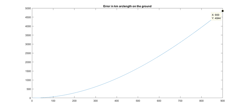
The model is a circular orbit, not an elliptical one. This has various implications for the velocity and altitude differences from reality. An analysis of the ground-track error was performed. The following plot tracks the error as the model diverges from ephemris data for a random pass of NOAA-18. Max error (for this pass) was only 4.8km after 15 minutes (max pass duration). Running a rough analysis pass, then following it up with a re-initialization of the model using the ephemris parameters at the point of minimum relative velocity should spread the error to the horizons and minimize the solution error.